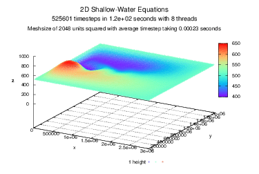
Saint-Venants Equations
Basic Fluid Representations
Basic Forms of Fluid Flow
Introduction to the Saint-Venant’s Equations
The Saint-Venant equations, or the “shallow-water equations”, are used to model free surface flows. In particular, the flows that it models tend to have greater horizontal length scales than flow depth. In regards to our fluid flow model, this implies that the cross section of the water source we are evaluating is significantly longer than it is deep, thus implying a “shallow” state. The equations use distributed flow routing, and thus focus on modeling the system with continuity and momentum equations. The system has the momentum equation setup of a dynamic wave, and can be applied to a variety of fluid models, from drops disturbing a still pond to pollution to tsunami modeling. This page should provide a foundation for understanding the Saint-Venants equations through their typical forms, a simplified version, and then applied to demonstrate sediment interactions in the water.
Assumptions of the Saint-Venant’s Equations
To reiterate, these equations do assume a “shallow” style cross sectional area. The equations thus represent the flow in a single dimension, with an incompressible fluid, and fixed boundaries. In other words, the water is viewed as flowing horizontally, and the channel is not considered to be affected by erosion within the context of the equation. Resistance is represented by Manning’s and/or Chezy’s equations. The bottom slope and streamline curvature are assumed to be relatively small, and vertical accelerations are considered negligible.
Use of the Continuity Equation
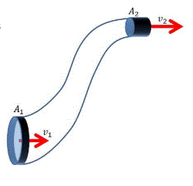
Continuity equations are used to describe the transport of quantities, in this case the transport of fluid. It describes the rate at which the fluid is entering the system, and assumes it exits at the same rate, while accumulating the fluid already contained in the system. To clarify, for the incompressible fluid in the Saint-Venant’s equations, the continuity equation states that the volume flux, composed of the cross sectional areas An and speeds vn of each entrance should be maintained at the exits.
A typical continuity equation incorporates density, but because of the fluid’s incompressible nature, its density is constant and the applicable continuity equation is purely of volume. Eliminating the density eliminates the divergence of the velocity field, which means there is no local volume dilation, and the it is thus the velocity that will be adjusting based off the exit’s size to ensure the exit flow rate is equivalent to the entrances.
Use of the Momentum Equation
The momentum equation serves as a restatement of Newton’s second law. Moving fluids apply forces as they interact with each other. The momentum equation does look different within the context of fluid dynamics, particularly because it can grow difficult to determine exactly what masses of the fluid should be considered. Also, because the density is determined to be constant, F = ma can essentially be rewritten as F= Qρ(v2-v1 ), with Q serving essentially as the area multiplied by the distance, and ρ representing the density.
The following are some examples of different forms of a momentum equation in fluid dynamics:
-
A kinematic wave has steep slope channels and no backwater (or obstruction blocking flow) effect. It is formed when the gravity and friction forces cancel out.
-
A diffusion wave forms when the pressure forces have substantial impact on the fluid.
-
A dynamic wave has mild slope channels and downstream control. It is more complicated, but can portray a wide variety of channel flow scenarios, from pressurized flow to backwater. Both the inertial and pressure forces tend to hold importance for dynamic waves.
General form of a momentum equation
vt + vvx + gyx - g(S - Sf) = 0
Dynamic
Diffusion
Kinematic
Friction Force Term
Gravity Force Term
Pressure Force Term
Convective Acceleration Term
Local Acceleration Term
Chezy's and Manning's Equations
These empirical equations are essentially used to approximate the average velocity of the flow. The general equation can be stated as thus:
v = C(Ri)
C = Chezy's constant
v = average velocity
R = hydraulic radius, which essentially functions like depth
i = hydraulic gradient, which relates the flow to the bottom slope
Manning then took Chezy's equation and ran further experiments, and found his empirical data to set the following equation for what Chezy had presented as a constant. His coefficient equation is considered more detailed and is considered the base formula for flow analysis.
C = (1/n) R
n = Manning's roughness coefficient
1/2
1/6
Most Common Form of Saint-Venant Equations
Continuity Equation:
At = - (vA)x + q
Momentum Equation:
(vA)t = - (v2A)x - Ag(hx + Sf) + qµ
Which can be expanded to:
vtA + vAt= -vx2A -v2Ax -Ag(hx + Sf) + qµ (momentum equation)
The above form assumes that h(x,t) is some function that is possible to evaluate from the cross section information.
What does the equation mean?
A = cross section (x,t)
Ax = the changing size of the cross section in regards to space (essentially, the shape of the bottom along certain points of space)
At = the speed at which the cross sectional area is changing based on the flow of water
v = water speed (x,t)
vx = speed changing along the course of space
vt = the horizontal acceleration of the water flow
q = in-and outflows
µ= speed of the lateral in and outflows
h = water height above sea level
Sf = friction slope
g =gravity
The continuity equation here shows that the cross sectional area changes over time based off the in and out flows of fluid, as well as the the shape of the cross section in regards to space scaled by the speed of the water, and the change of the speed along the course of space scaled by the overall cross sectional area.
The momentum equation here focuses on the cross sectional area scaled by the horizontal acceleration of the flow, and the cross sectional area changing over time scaled by the speed of the water. These two terms are set equivalent to the in and out flows, the momentum flow across the control volume, the speed as it changes over space squared scaled by the cross sectional area, and the shape of the area over space scaled by the the value of the water speed squared.
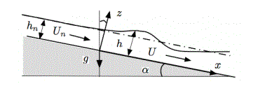
Second Form of the Equation
The following equations are essentially equivalent to the equation above in function, but incorporates an angle. To avoid redundancy, I will simply clarify certain variables.
ht + (vh)x = 0
vt + vvx + ghxcos(α) = gsin(α)(1/2)Cf(h,v)(v|v|/h)
h(x,t)= flow depth
v(x,t) = vertically averaged velocity
g = gravity
Cf (h,U) = dimensionless drag coefficient, specifically utilizing the Chezy’s or Manning’s equations
(v|v|/h) = seems to function like Froude's number, which essentially describes the energy state
α= bottom angle with the horizontal plate
Simplified Version
Assumptions for simplifications:
-
a rectangular cross-section A = By
-
no lateral in- or outflows (q = 0)
lead to the simplified equations:
yt = -(vy)x
vt = -vvx - gyx + g(S-Sf)
Where
B = constant width
S= slope of the river bed
Sf = friction slope
g = gravity
y = water height with respect to the river bed
yt = the speed at which the water height is changing
yx = essentially the changing steepness of the height
v = speed of the moving water
vx = speed changing along the course of space
vt = the horizontal acceleration of the water flow
The continuity equation shows that, in this simplified system, the speed at which the water height is changing depends on the speed over the space scaled by the current height, and the changing steepness scaled by the speed of the water.
The horizontal acceleration of the water flow adjusts with the changing steepness of the height of the water scaled by the gravity force, the change of the speed across the course of the space scaled by the general speed, and the force of gravity on the slope and friction slope.
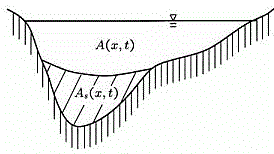
Application: Sediment Pollution
(Af + As)t = -(Qf)x + qf
(A + As)t = -Qx +qw+qf
Qt + (vQ)x = - Ag(hx+Sf) + µ(qw+qf)
where
Aw = cross-section area of flowing water(w)
Af= cross-section area of flowing sediment
As = cross section area of deposited sediment
g = gravity
h(x,t) = water height above sea level
ht =
hx =
v = water speed
vt = the horizontal acceleration of the water flow
vx = speed changing along the course of space
Sf = friction slope
Q= discharge Q = v A
Qw = v Aw
Qf = v Af
qw,f = lateral water (w) and sediment (f) inflows and outflows
µ= speed of the lateral in and outflows
Sediment is a very interesting type of pollution to model, because its behavior adjusts based upon the strength of the flow itself. It can either be carried by the fluidic forces, sink to the bottom, or disperse in a combination of both.
This system uses partial differential equations to break down the mass into sediment and water components. The lateral inflows and outflows are composed of purely water and sediment, which is then discharged at the rate of the velocity of the flow. The cross section, however, also includes sediment that is is not flowing, and is thus considered as sinking to the bottom.
The sediment continuity equation essentially shows that the cross section areas of the overall sediment change over time in accordance with the varying discharge of flowing sediment, along with the lateral in or outflow of sediment. The systematic continuity equation shows that the total cross sectional area and the amount of deposited sediment adjusts over time in relation to the systematic discharge and the in and out flows of both water and sediment.
The momentum equation highlights that the general discharge (the water speed by the overall cross sectional area) over time, the spatial discharge scaled by the velocity, and the change of the speed over space scaled by the general discharge change in relation to the water height and friction slope scaled by the cross sectional area and gravity forces and the in and out flows of water and sediment throughout the system, scaled by their own speed.